
Part 2 of Understanding Your Workflow Capacity

Timothy D. Cooper, Chief Architect,
NCP Solutions
In my previous post, I described the components of workflow capacity and the need to identify the constraints on each component. In this post, I move on to discuss methods for measuring workflow capacity so that workflow can be managed efficiently.
Determining the capacity of each workflow component can be difficult. Ideally the throughput of each workflow component is logged (in real time) into a database where it can be aggregated and normalized. If throughput is not being logged, this information can be gathered by running controlled tests. Below is an example of a typical capacity matrix. While gathering this information may be difficult, it will provide the core data needed to model job throughput.
| Component | Metric | Per Minute | Per Hour |
| Extract, Transform and Load | Records per minute | 12,000 | 720,000 |
| Address Cleansing / PreSort | Documents per minute | 2,400 | 144,000 |
| Composition | Images per minute | 1,200 | 72,000 |
| Electronic Services | Images per minute | 1,200 | 72,000 |
| Images per minute | 1100 | 36,000 | |
| Finishing | Sheets per minute | 600 | 36,000 |
Figure 1. Capacity Matrix
Now that we know the capacity of each component within our workflow, we are now ready to model an actual production job.
Job Capacity Attributes
The receipt of a file typically triggers the creation of a unit of work we will refer to as a Job. For purposes of this discussion, we will assume the file contains multiple records per document and the number of pages (sheets) within each mail piece can vary from 1 to 10 pages.
At file receipt; we may only know the size of the file and the Service Level Agreement (SLA) usually defined in days (1 day turn, 2 day turn, etc.). To gather the capacity attributes that will affect downstream processing, we must analyze the contents of the file. This can be accomplished using some type of Extract, Transform and Load process. Once a file goes through this process; we can determine the following capacity Attributes:
- SLA
- Number of records
- Number of documents or mail pieces
At this point, in a transaction printing or direct mail environment, it is common to run the address lines from the file through address hygiene solutions, DPV, LACS and possibly zip code presort to optimize for postal discounts.
Further pre-composition processing will provide the remaining two capacity attributes needed by the simple workflow process.
- Number of sheets (physical pages)
- Number of images (logical pages)
With these five Job attributes; we now have the core information needed by our workflow system to determine if we have the capacity to meet the SLA. Below is an example Job with the attribute metrics defined that affect capacity.
| Job Attribute | Attribute Metric |
| Processing SLA in Minutes | 240 |
| Documents / Mail Pieces | 19,900 |
| Records | 417,900 |
| Sheets | 23,880 |
| Images | 28,656 |
Figure 2: Job Attributes and Metrics
Note that in this example, the SLA is 24 hours. In order to meet that SLA, the workflow system must have the composed documents ready to print within 4 hours to provide Operations the time they need to print and mail the Job.
Model Capacity
We now have everything we need to determine if we have the capacity required to meet an SLA. The following three examples, based on Figure 3: Current Workflow Capacity, will illustrate how minor changes in Job attributes can surface a different constraint.
Please note that all examples will use a workflow system with the following capacity metrics. Only Job attributes will be modified between examples.
|
Component |
Metric |
Per minute |
Per Hour |
|
Extract, Transform and Load |
Records per minute |
12,000 |
720,000 |
|
Address Cleansing |
Documents per minute |
2,400 |
144,000 |
|
Composition |
Images per minute |
1,200 |
72,000 |
|
Electronic Services |
Images per minute |
1,200 |
72,000 |
|
Printing |
Images per minute |
1,100 |
66,000 |
|
Finishing |
Sheets per minute |
600 |
36,000 |
Figure 3: Current Workflow Capacity
Example 1:
Based upon a Job with the following attributes, Finishing will be the first constraint; however, the Job will complete within SLA. Comparing the Documents to Sheets attributes, most of these mail pieces are 1 page documents.
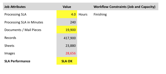
Figure 4: Job Attributes of Example 1
Example 2:
Based upon a Job with the following attributes, Printing will be the first constraint; however Job will complete within SLA. The only change between Example 1 and 2 is the number of images increased. The increase in the number of images results in more duplex printing; which requires additional time on the printers. NOTE: The assumption in this workflow is duplex printing requires a 2nd pass at the printer.
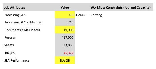
Figure 5: Job Attributes of Example 2
Example 3:
Based upon a Job with the following attributes, the constraints did not change. Printing continues to be the top constraint. The basic change between Example 2 and 3 is the increase in the number of mail pieces that resulted in the SLA being missed. In this example; the entire workflow is ranked top to bottom; starting with the largest constraint (Printing) to the smallest constraint (Address Cleansing).
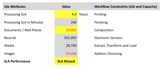
Figure 6: Job Attributes of Example 3
Summary
The intent of the above tables is to illustrate the complexity around determining and managing your workflow resources. Knowing your next bottleneck and the corresponding job attributes that will trigger that bottleneck is essential to meeting SLA performance expectations; especially in a time of growth and expansion.
Waiting until you hit a constraint is disastrous. Adding capacity (depending on the workflow component) often takes several months. Know your workflow metrics.